Image processing in neuroimaging applications

Detrending

Overview

Teaching: 25 min
Exercises: 10 min

Questions

How do we eliminate trends in our data?

Why are linear models useful?s

Objectives

Detrend image data with a linear model

Use a linearized quadratic model to fit second order effects

Using the spatial relationships in image processing

In the first example of image processing operations that we will explore, the spatial relationships between voxels will be made rather explicit. We will use the spatial coordinates to remove spatial trends from the data.

Our data contains spatial bias

As we saw in the last part, MRI data often contains spatial biases. Some of these may be due to physiological factors, such as differences in the T1 time-constant between different parts of the brain. But some of these represent “nuisance factors” that should be eliminated as a first step in the analysis of the image.

For example, the image is brighter in the back of the head of this participant than in the front. This often happens when the head is placed closer to the measurement coils that are at the bottom of the coil, closer to the occipital cortex. We can also see that the center of the brain is darker than the more external parts, also presumably due to the distance of these parts from the measurement coils.

To model this spatial bias and remove it, we will assume that changes across the entire extent of the image are due to bias.

Modeling linear bias and detrending

A linear spatial bias can be thought of as another 3D volume that coexists in the same space as our data. This bias field can be modeled as a combination of of biases on the x, y and z dimensions.

We’ll use the np.meshgrid function to create volumes that contain the 3D functions:

$vol(x,y,z) = x \\ vol(x,y,z) = y \\ vol(x,y,z) = z \\$

x,y,z = np.meshgrid(range(-T1w_data.shape[0]//2, T1w_data.shape[0]//2),
                    range(-T1w_data.shape[1]//2, T1w_data.shape[1]//2),
                    range(-T1w_data.shape[2]//2, T1w_data.shape[2]//2), indexing='ij')

To clarify, let’s also create a little function that will help us view these volumes:

def show_volumes(volume_list):
    fig, ax = plt.subplots(1, len(volume_list))
    for idx in range(len(volume_list)):
        this = volume_list[idx]
        ax[idx].matshow(this[:, :, this.shape[-1]//2], cmap='bone')
        ax[idx].axis('off')
    fig.set_size_inches([14, 5])
    return fig

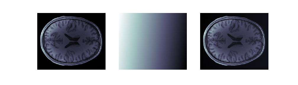
For example, the following should show sections through the T1-weighted data, as well as through each one of these volumes:

fig1 = show_volumes([T1w_data, x, y, z])
fig2 = show_volumes([T1w_data.T, x.T, y.T, z.T])

Linear trends

You can see that in the top row, the x volume changes gradually along the right-left dimension of the participants head. The y volume changes gradually along the anterior-posterior dimension. The z volume doesn’t change at all (why?). Similarly, in the second row, the z and y volumes change, while the x volume remains constant along this entire slice.

Mathematically, the bias field can be described as a linear combination of these three volumes:

$data_{measured} = data_{true} + bias$ $bias = data_{measured} - data_{true}$

where

$bias = \beta_1 x + \beta_2 y + \beta_3 z$

Another way of saying this is that all linear bias fields are spanned by the basis set comprising x, y and z.

Next, we are going to make a simple assumption that in the lack of any spatial bias, the data would have a more-or-less constant value across space. That is, we assume that for unbiased data,

$\beta_1 = \beta_2 = \beta_3 = 0$ .

This seems like a strange assumption to make, but it makes sense when you think of the fact that we expect the brain to be more or less symmetrical (it’s not supposed to be much brighter in any particular direction), and given the spatial scale of the functions we are using for debiasing.

Even if you feel uncomfortable with this assumption, you might want to remember that the T1-weighted measurement is just that: a non-quantitative weighted measurement that is affected by T1, but not directly reflective of. If subsequent image processing operations are made simpler by this detrending, it might be worth ignoring actual biological differences (e.g. white matter with T1 that is slightly different in frontal cortex, relative to other lobes) in the service of these other steps.

But this allows us to rewrite the above function as:

$data_{measured} = \beta_1 x + \beta_2 y + \beta_3 z$

Then, To find the values of ${\bf \beta}$ we start by unraveling the data and the regressors into one-dimensional vector form, using the np.ravel function:

regressors = np.vstack([np.ravel(x), np.ravel(y), np.ravel()]).T
data = np.ravel(T1w_data.ravel)
data.shape, regressors.shape

((21023600,), (21023600, 3))

The shape of the unravelled data is the product of the x, y and z dimensions of the data

The problem we are now trying to solve can be written as the following set of linear equations:

$\begin{pmatrix} T1_{0,0,0} \\ T1_{0,0,1} \\ \vdots \\ T1_{0, 0, N_z} \\ T1_{0, 1, 0} \\ T1_{0,1,1} \\ \vdots \\ T1_{1,0,0} \\ T1_{1,0,1} \\ \vdots \\ T1_{N_x, N_y, N_z} \end{pmatrix} = \begin{pmatrix} x_{0,0,0} & y_{0,0,0} & z_{0,0,0} \\ x_{0,0,1} & y_{0,0,1} & z_{0,0,1}\\ \vdots & \vdots & \vdots \\ x_{0, 0, N_z} & y_{0, 0, N_z} & z_{0, 0, N_z} \\ x_{0, 1, 0} & y_{0, 1, 0} & z_{0, 1, 0} \\ x_{0,1,1} & y_{0,1,1} & z_{0,1,1} \\ \vdots & \vdots & \vdots \\ x_{1,0,0} & y_{1,0,0} & z_{1,0,0} \\ x_{1,0,1} & y_{1,0,1} & z_{1,0,1}\\ \vdots & \vdots & \vdots \\ x_{N_x, N_y, N_z} & y_{N_x, N_y, N_z} & z_{N_x, N_y, N_z} \end{pmatrix} \begin{pmatrix} \beta_1 \\ \beta_2 \\ \beta_3 \end{pmatrix}$

These equations can be solved for ${\bf \beta}$ with an Ordinary Least Squares solution. This is implemented in scipy.linalg as lstsq:

import scipy.linalg as la
# la.lstsq?  # Get help about this function

solution = la.lstsq(regressors, data)

Because the solution is a tuple with a variety of information about the solution, we’ll just extract out only the first element:

beta_hat = solution[0]

Inverting the equation gives us an estimate of the linear trend, but it still has the unravelled shape:

linear_trend = np.dot(regressors, beta_hat)
linear_trend.shape

(21023600,)

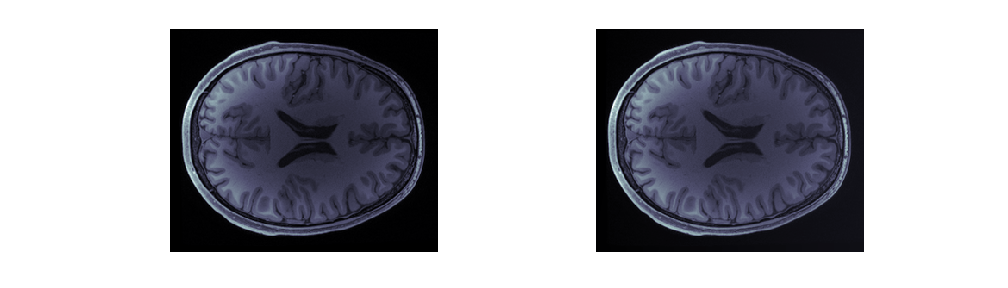
We reshape it back to the correct shape, and remove it from the data for a detrended volume, which we can examine side-by-side with the original data:

linear_trend = np.reshape(linear_trend, T1w_data.shape)
T1w_linear_detrend = T1w_data - linear_trend
fig = show_volumes([T1w_data, linear_trend, T1w_linear_detrend])

Linear detrending

Let’s write a function to codify this entire process:

def detrend(data, regressors):
    regressors = np.vstack([r.ravel() for r in regressors]).T
    solution = la.lstsq(regressors, data.ravel())
    beta_hat = solution[0]
    trend = np.dot(regressors, beta_hat)
    detrended = data - np.reshape(trend, data.shape)
    return detrended, beta_hat

This simplifies the process to:

T1w_linear_detrend, beta_hat = detrend(T1w_data, [x, y, z])

fig = show_volumes([T1w_data, T1w_linear_detrend])

Linear detrending

“Detrending”

Note that “detrending” is often used in a similar manner in neuroimaging to remove temporal biases. Here we are rather performing a spatial detrending operation

One way to understand the nature of the bias field is to examine the values of the coefficients that were found in the solution to the linear equations.

fig, ax = plt.subplots()
ax.bar(np.arange(beta_hat.shape[0]), beta_hat)
ax.set_xticks(np.arange(beta_hat.shape[0]) + 0.4)
ax.set_xticklabels(['x', 'y', 'z'])
ax.set_ylabel('beta')

Linear betas

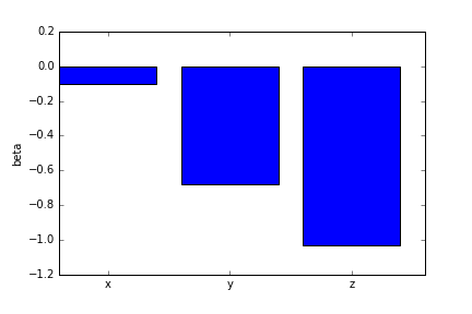
We can see that there is almost no right-left bias field. Indeed, there is some anterior-posterior bias and an even more substantial superior-inferior bias.

What can we do with the remaining interior-exterior bias?

Examining the images, we can see that the detrending has removed some of the biases in the data, but there is still a clear interior-exterior bias.s What could we do to help mitigate this additional bias?

Removing additional bias with a linearized model

The linear model we have seen so far does manage to get rid of some of the bias, but what can we do to get rid of the interior-exterior bias?

To do so, we add to our bias-field model quadratic functions, to augment the linear trends that we already have included:

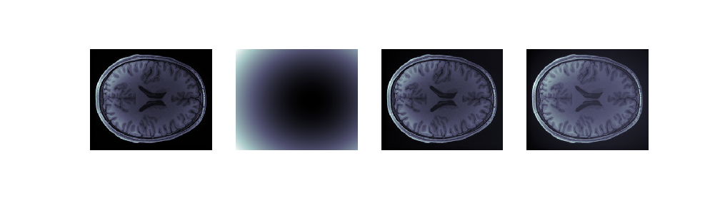
x_sq = x**2
y_sq = y**2
z_sq = z**2
fig = show_volumes([x_sq, y_sq, z_sq])

Quadratic functions

These functions allow us to model second order trends in the data. Perfect for modeling trends like a center-out brightening.

This model has more parameters and a wider design matrix:

$data = \beta_1 {\bf x} + \beta_2 {\bf y} + \beta_3 {\bf z} + \beta_4 {\bf x^2} + \beta_5 {\bf y^2} + \beta_6 {\bf z^2}$ $\begin{pmatrix} {\bf T1w} \\ \vdots \end{pmatrix} = \begin{pmatrix} {\bf x} && {\bf y} && {\bf z} && {\bf x^2} && {\bf y^2} && {\bf z^2} \\ \vdots && \vdots && \vdots && \vdots && \vdots && \vdots \end{pmatrix} \begin{pmatrix} \beta_1 \\ \beta_2 \\ \beta_3 \\ \beta_4 \\ \beta_5 \\ \beta_6 \end{pmatrix}$

We sometimes call this kind of a model a “linearized” model, because we have inserted non-linear equations into the form of the general linear model.

Using our detrend function, we can construct and solve the augmented model:

T1w_data_detrended_quad, beta_hat = detrend(T1w_data, [x, y, z, x_sq, y_sq, z_sq])
fig = show_volumes([T1w_data, quadratic_trend, T1w_data_detrended, T1w_data_detrended_quad])

Quadratic detrending

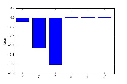
fig, ax = plt.subplots()
ax.bar(np.arange(beta_hat.shape[0]), beta_hat)
ax.set_xticks(np.arange(beta_hat.shape[0]) + 0.4)
ax.set_xticklabels(['x', 'y', 'z', '$x^2$', '$y^2$', '$z^2$'])
ax.set_ylabel('beta')

Quadratic betas

Should we keep going?

We could augment this model of the bias further with additional functions ($x^3$, $x^4$, etc.), but should we really keep going? At some point, the functions that we use will start picking up the interesting spatial variation in the data, rather than the large-scale bias. So, we can’t just keep going with this.

When is it enough?

In some conditions, you might be able to determine empirically when you should stop the process of augmenting a model. A variation of this principle is demonstrated in the temporal domain in this paper

XXX

XXX

Key Points

Linear models are useful to represent the images in a concise and computationally expedient manner

Linearized models are used to fit more complex models using the same mathematical framework