Image processing in neuroimaging applications

Segmentation

Overview

Teaching: 15 min
Exercises: 0 min

Questions

How can we segment an image into different sections?

Objectives

Understand the prinicples behind the median Otsu segmentation algorithm

Use scikit-image to perform histogram-based segmentation

Use scikit-image to perform edge-based segmentatio

Segmentation is a basic operation in image processing. Very often, we will want to use image information in order to differentiate between different parts of the image as belonging to different objects, or different classes.

We will talk about two different ways of segmenting an image. Neither of them will be particularly good, but they will at least teach you how to think about image processing.

We will use scikit-image to perform these operations

Histogram-based segmentation

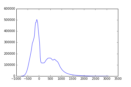
One way of segmenting an image is to look at the histogram of the pixel intensities and differentiate between classes. Let’s examine the histogram:

hist, bin_centers = exposure.histogram(T1w_data.ravel())
fig, ax = plt.subplots(1)
ax.plot(bin_centers, hist)

Pixel histogram

There are several different methods that use the histogram to perform segmentation. We’ll closely examine one of these algorithms that is a classic algorithm designed by Nobuyuki Otsu, a Japanese Engineer, back in the 1970’s

Otsu’s method for segmentation

https://en.wikipedia.org/wiki/Otsu%27s_method

Assumes there are two classes of voxels: background and foreground. The algorithm attempts to set a threshold in the histogram, such that the variance within each class of the image is minimized.

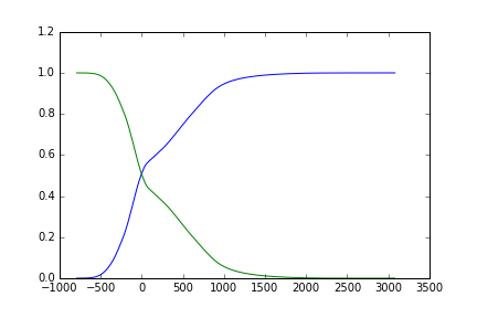
The class probabilities as a function of the threshold $t$ are the cumulative sums of the distributions up to that point:

$w_1(t) = \sum_{i=1}^{t-1} \frac{hist(i)}{L}$ $w_2(t) = \sum_{i=t}^{L-1} \frac{hist(i)}{L}$

where L is the total number of pixels

That looks like this:

# Normalize the histogram to sum to 1:
hist = hist.astype(float) / np.sum(hist)

# class probabilities for all possible thresholds
weight1 = np.cumsum(hist)
weight2 = np.cumsum(hist[::-1])[::-1]

Plotting this:

fig, ax = plt.subplots(1)
ax.plot(bin_centers, weight1)
ax.plot(bin_centers, weight2)

Weights

Recall that we are trying to minimize the intra-class variance:

Otsu’s method relies on finding a threshold that minimizes the intra-class variance:

$\sigma^2_w = w_1 \sigma^2_1 + w_2 \sigma^2_2$

But minimizing intra-class variance is equivalent to maximazing inter-class

Importantly, minimizing intra-class variance, is equivalent to maximizing inter-class variance.

That is becauase:

$\sigma^2 = \sigma^2_w + \sigma^2_b$

That’s because the sum of squares is always constant:

$\sigma^2_b = \sigma^2 - \sigma^2_w$

The inter-class variance can be written as:

$w_1 (\mu_1 - \mu)^2 + w_2 (\mu_2 - \mu)^2 = w_1 w_2 (\mu_1 - \mu_2)^2$

Where

$\mu_1 = \sum_{i}^{t-1} \frac{i p(i)}{w_1}$ $\mu_2 = \sum_{t}^{L-1} \frac{i p(i)}{w_2}$

The advantage of this formulation is that it can be written in code that can run fast.

We start by setting the means of the background/foreground for all possible thresholds:

# class means for all possible thresholds
mean1 = np.cumsum(hist * bin_centers) / weight1
mean2 = (np.cumsum((hist * bin_centers)[::-1]) / weight2[::-1])[::-1]

Plotting this:

means

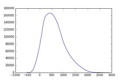
And calculate the inter-class variance:

# The last value of `weight1`/`mean1` should pair with zero values in
# `weight2`/`mean2`, which do not exist.
variance12 = weight1[:-1] * weight2[1:] * (mean1[:-1] - mean2[1:]) ** 2

fig, ax = plt.subplots(1)
ax.plot(bin_centers[:-1] ,variance12)

Intraclass=variance

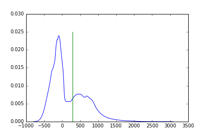
To find the threshold value that marks the distinction between the two classes we detect the maximum of this function:

idx = np.argmax(variance12)
threshold = bin_centers[:-1][idx]

Visualizing this threshold, with respect to the histogram:

fig, ax = plt.subplots(1)
ax.plot(bin_centers, hist)
ax.plot([threshold, threshold], [0, ax.get_ylim()[1]])

Intraclass=variance

We can create binary mask based on this value:

binary = T1w_data >= threshold
fig, ax = plt.subplots()
ax.matshow(binary[:, :, binary.shape[-1]//2], cmap='bone')

Otsu Mask

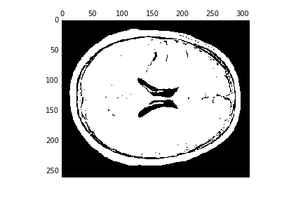
This looks like it can (in this case, easily…) separate background from foreground. Can we do any better with a histogram-based segmentation. For example, do you think that it would be possible to strip the skull off with this type of algorithm?

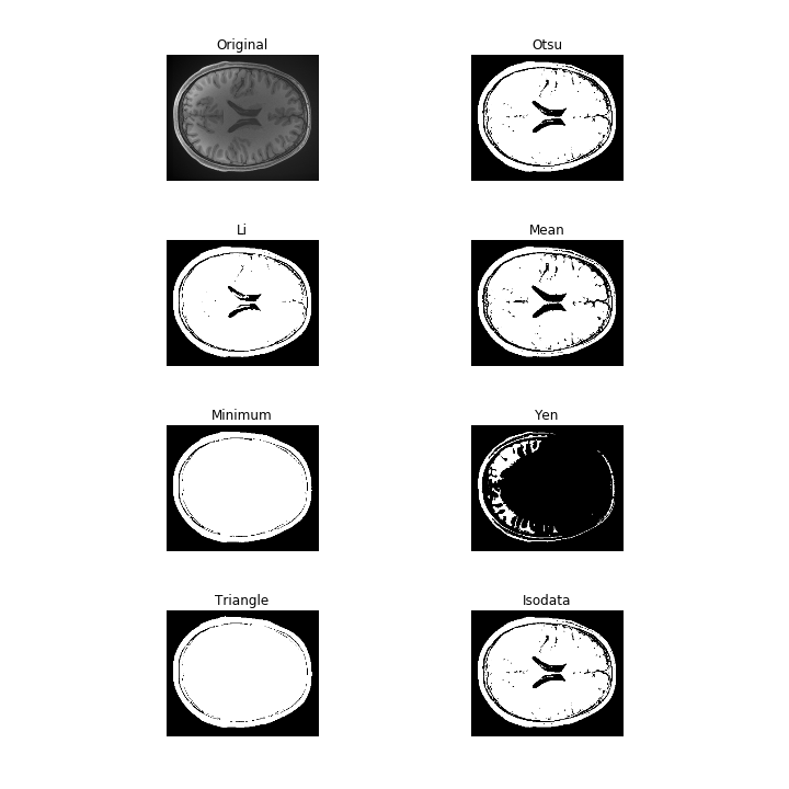
The filters module in scikit-image contains a variety of thresholding algorithms. You can try all of them by running:

from skimage import filters
fig, ax = filters.thresholding.try_all_threshold(T1w_data[:, :, T1w_data.shape[-1]//2])
fig.set_size_inches([10, 10])

skimage threshold filters

Edge-based segmentation

Another way to segment an image is based on detecting edges in the image, and filling between these edges. Detecting images is part of a larger set of operations that can be done on image: detecting image features.

The module that does these operations is skimag.feature:

from skimage import feature

Unfortunately, these algorithms usually only work on 2D images, so we’ll work on one slice from now on:

im = T1w_data[:, :, T1w_data.shape[-1]//2]

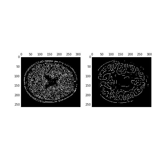
A classic edge detection algorithm is the Canny filter.

The performance of the algorithm depends strongly on the sigma parameter, which corresponds to the width of a Gaussian smoothing kernel that is applied to the image before edges are detected.

edges1 = feature.canny(im, sigma=1, mask=binary[:, :, binary.shape[-1]//2])
edges4 = feature.canny(im, sigma=4, mask=binary[:, :, binary.shape[-1]//2])
fig, ax = plt.subplots(1, 2)
ax[0].matshow(edges1, cmap='bone')
ax[1].matshow(edges4, cmap='bone')

Canny filter

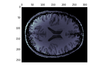
Scikit image works well together with the image processing tools that are implemented in scipy. We use these to dilate the edges slightly and fill the holes in the image:

from scipy import ndimage as ndi
dilated = ndi.binary_dilation(edges1, iterations=1)
fill_brain = ndi.binary_fill_holes(dilated)

brain = np.zeros(im.shape)
brain[fill_brain] = im[fill_brain]
fig, ax = plt.subplots(1)
ax.matshow(brain, cmap='bone')

This doesn’t work great:

Fill from Canny

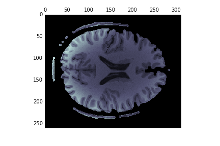
Another approach is to start the edge-based segmentation with the results of the histogram-based segmenation:

edges = feature.canny(binary[:, :, binary.shape[-1]//2],
                      sigma=1, mask=binary[:, :, binary.shape[-1]//2])

dilated = ndi.binary_dilation(edges, iterations=1)
fill_brain = ndi.binary_fill_holes(dilated)
brain = np.zeros(im.shape)
brain[fill_brain] = im[fill_brain]
fig, ax = plt.subplots(1)
ax.matshow(brain, cmap='bone')

This works much better

Fill from Canny

Conclusions

You can use any one of these approaches, but you will find that often it is necessary to construct a pipeline of image operations: filtering, segmentation, feature-detection etc. in order to process your image and detect.

Key Points

There are three (at least) different ways to perform segmentation

The first uses the histogram of the pixel gray values

The second detects edges and fills between them